DFT analysis of FIR filters

Contents

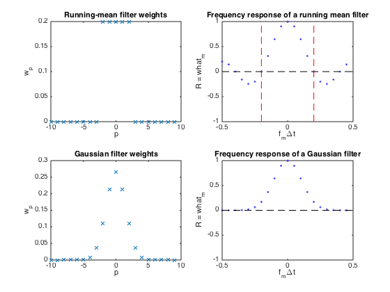
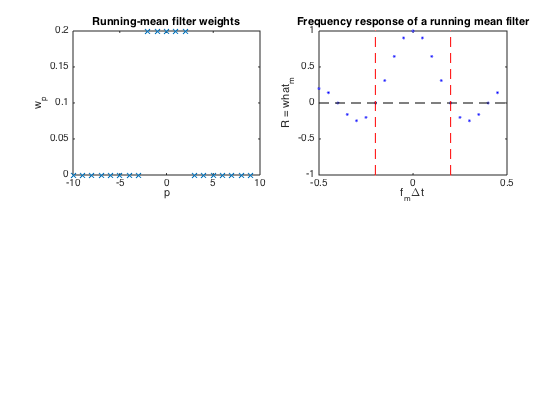
Running-mean filter

N = 20;  % Length of time series
Nav = 5;  % Number of samples to average across (should be odd)
P = (Nav-1)/2;

% Define weight vector for running mean filter and take DFT
w = [ones(1,P+1) zeros(1,N-Nav) ones(1,P)]/Nav;
what = fft(w);
M = [0:(N/2-1) -N/2:-1];

% Plot filter weights

clf
subplot(2,2,1)
plot(M,w,'x')
xlabel('p')
ylabel('w_p')
title('Running-mean filter weights')

% Plot frequency response.  The filter zeroes out a sinusoidal signal of
% period Nav*dt, whose corresponding freq is at vertical dashed red lines.

subplot(2,2,2)
plot(M/N,what,'b.',[-0.5 0.5],[0 0],'k--',...
    (1/Nav)*[1 1],[-1 1],'r--',(1/Nav)*[-1 -1],[-1 1],'r--')
xlim([-0.5 0.5])
ylim([-1 1])
xlabel('f_m\Deltat')
ylabel('R = what_m')
title('Frequency response of a running mean filter')

% The running-mean filter has strong 'side-lobes' that pass high-frequency
% signals that are outside the desired pass-band. Thus, despite its
% simplicity, this filter is easily outperformed.

Warning: Imaginary parts of complex X and/or Y arguments ignored 

Gaussian smoother

% Define weight vector for running mean filter and take DFT

Pg=1.5; % Set filter width to have a similar pass-band to running-mean
w = exp(-M.^2/(2*Pg^2));
w = w/sum(w);  % Normalize so low-pass response is 1
what = fft(w);
M = [0:(N/2-1) -N/2:-1];

% Plot filter weights...w could be truncated at p = +/- 3*Pg without
% significant loss of accuracy.

subplot(2,2,3)
plot(M,w,'x')
xlabel('p')
ylabel('w_p')
title('Gaussian filter weights')

% Plot frequency response.  The filter zeroes out a sinusoidal signal of
% period Nav*dt, whose corresponding freq is at vertical dashed red lines.

subplot(2,2,4)
plot(M/N,what,'b.',[-0.5 0.5],[0 0],'k--')
xlim([-0.5 0.5])
ylim([-1 1])
xlabel('f_m\Deltat')
ylabel('R = what_m')
title('Frequency response of a Gaussian filter')

% The Gaussian filter does not have side-lobes so is less susceptible to
% spectral leakage.  However, it still does not have a very sharp frequency
% cutoff at the edge of its passband.

Warning: Imaginary parts of complex X and/or Y arguments ignored 

Published with MATLAB® R2014b